Rich Feature Hierarchies for Accurate Object Detection and Semantic Segmentation

总结

• 新的detection方法的特点
  • 利用了高拟合能力的卷积神经网络
  • 缓解了训练detection任务数据量少的问题

物体定位问题

旧方案：

• 当成回归问题做——效果不好
• 用滑动窗口做——新的数据集图片比较大，不适合

新方案：

• (用selective search)生成proposals
• 通过CNN对每个proposals生成固定长度的特征向量
• 用多个SVM判定向量是否属于特定类别
• 非极大值抑制筛选最终结果

数据量少的问题

旧方案：

• 先使用无监督训练，然后有监督fine-tuning

新方案：

• 先用大量的无关classification数据训练网络初始参数
• 然后用特定类别有监督fine-tuning
• 迁移学习思想

可拓展性

• 生成proposal的时候是类别无关的
• CNN抽取特征的时候是类别无关的
• 最后的SVM判别是和类别数量相关，但只是线性相关
• 非极大值抑制过程也是线性相关
• 所以在目标类别很多的时候依旧能保证高效率，而不用去做近似计算

训练细节

CNN 预训练

之就用classification的数据训练就行
这个阶段训练的是模型对于图像信息的泛化抽取能力

CNN fine-tuning

• 把预训练的最后一层替换为目标类别数+1（背景算作一个类别）的分类层
• 所有和标记框IoU >= 0.5的proposal当做标记框所在类别的正样本否则当做负样本
• 学习率是预训练阶段的十分之一（0.001）
• 用32个正样本和96个负样本组成一个128的batch（这个比例主要是因为正样本少）

特征分类

• 比fine-tuning的样本筛选更加严格
  • 只有标记框抽取出来的特征当做正样本
  • 与标记框IoU低于0.3(grid search出来的)的当做负样本
  • IoU大于0.3但是小于1的扔掉

为什么两次正负样本的选择标准不同？

训练CNN的时候需要的数据量比较大 fine-tuning阶段对于正样本的选取标准是一种对于标记数量不足的妥协，IoU高于0.5的都当做正样本的话，相对于标记框的数量增长了30倍，虽然数据精度下降但是最终效果反而更好

为什么不用CNN直接分类？

fine-tuning的样本选取方式不适合用于精确定位位置，所以单独训练模型去干这个事
训练数据要求尽可能干净，所以有了更严格的样本选取标准
这样一来数据量又不够了，好在SVM对于数据量少的容忍度相对较高——引入最大间隔概念，使用结构风险而非经验风险来作为损失函数
所以选择SVM作为最后的分类模型

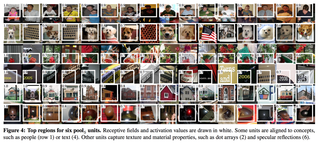
特征可视化

• 选定一个特征（本文选取的是$pool_5$里的特征）
• 用大量的proposal过神经网络，得到这个特征的值
• 按特征值从大到小排列
• 非极大值抑制筛选proposal
• 把较大的proposal输出即为此特征的抽取信息的直观表现

分类特征值选择

• CNN最后的抽象特征有多层，本文对用不同的特征作为分类特征做了实验
• 如果没有经过fine-tuning那么用靠前网络层的更好($fc_6 > fc_7$)
• 经过fine-tuning的就用后面层作为分类特征值

网络结构选择

CNN作为特征抽取器，其结构对于最后的效果有非常大的影响

用了新的VGG网络进行对比，效果确实好，但是算的确实慢

bounding-box回归

借助错误分析工具可知，detection位置错是mAP低的主要原因

所以单独训练一个模型去修正位置问题

• 用中心点x, y坐标，方框长和宽四维数据去定义边框
• 训练四个映射，把四维数据映射为真实值
• 用CNN $pool_5$的值代表proposal信息
• 采用LR模型
• 只把proposal和真实边框IoU大于等于0.6的当做训练数据
• 正则化参数很重要

目标函数：

$$w_* = \underset {\hat w_*} {argmin} \sum^N_i(t^i_* - \hat w^T_*\phi_5(P^i))^2 + \lambda ||\hat w_*||^2$$

与OverFeat对比

只有两个区别

• OverFeat用的是multi-scale pyramid而不是selective search
• OverFeat是为每个类别分别训练一个bounding-box regression模型

VOC测试结果

• time: 13000ms
• VOC 2010: 53.7%
• VOC 2011&2012: 53.3%
• VOC 2013: 31.4%

Abstract

propose a detection algorithm:

• one can apply high-capacity convolutional neural networks (CNNs) to bottom-up region proposals in order to localize and segment objects
• when labeled training data is scarce, supervised pre-training for an auxiliary task, followed by domain-specific fine-tuning, yields a significant performance boost

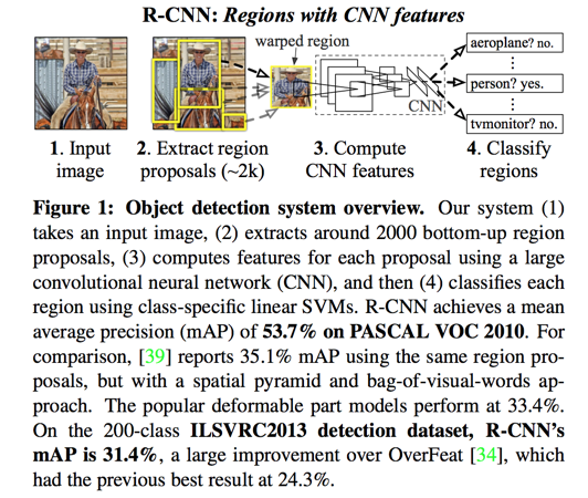
RCNN: Regions with CNN features

Introduction

we focused on two problems:

• localizing objects with a deep network
• training a high-capacity model with only a small quantity of annotated detection data

localizing objects with a deep network

old way:

• approach frames localization as a regression problem may not fare well in practice
• our network is too deep to use a sliding-window

new method:

• recognition using regions
• generate proposal
• extracts a fixed-length feature vector from each proposal using a CNN
• classifies each region with category-specific linear SVMs

scarce labeled data

old way:

• use unsupervised pre-training, followed by supervised fine-tuning

new method:

• supervised pre-training on a large auxiliary dataset
• followed by domain-specific fine-tuning on a small dataset

Object Detection with R-CNN

three modules:

• generates category-independent region proposals
• a large convolutional neural network that extracts a fixed-length feature vector from each region
• a set of class-specific linear SVMs

module design

region proposals

use selective search to enable a controlled comparison with prior detection work

use fast mode of selective search

feature extraction

use AlexNet

transformations

• isotropically scales
  • with context(B)
  • without context(C)
• anisotropically scales(D)

The amount of context padding (p) is defined as a border size around the original object proposal in the transformed input coordinate frame

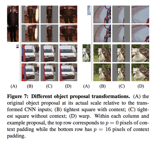
warping with context padding (p = 16 pixels) outperformed

test-time detection

given all scored regions in an image, we apply a greedy non-maximum suppression

run-time analysis

two properties make detection efficient:

• all CNN parameters are shared across all categories
• the feature vectors computed by the CNN are low-dimensional

13s/image on a GPU or 53s/image on a CPU

scalable:

• CNN feature are class-independent
• The only class-specific computations are dot products

this analysis shows that R-CNN can scale to thousands of object classes without resorting to approximate techniques

training

supervised pre-training

using image-level annotations only (bounding- box labels are not available for this data)

domain-specific fine-tuning

continue CNN training using only warped region proposals

the last layer is randomly initialized (N + 1)-way classification —— where N is the number of object classes, plus 1 for background

We treat all region proposals with ≥ 0.5 IoU overlap with a ground-truth box as positives for that box’s class and the rest as negatives

learning rate 0.001

In each SGD iteration, we uniformly sample 32 positive windows (over all classes) and 96 background windows to construct a mini-batch of size 128

object category classifier

Question:

• how to label a region that partially overlaps ground-truth?

Answer:

• We resolve this issue with an IoU overlap threshold
• negatives: proposal regions which IoU below threshold are defined as negatives
• positives: defined simply to be the ground-truth bounding boxes for each class
• threshold is 0.3 selected by a grid search
• proposals that fall into the grey zone (more than 0.3 IoU overlap, but are not ground truth) are ignored

Positive vs. negative examples and softmax

Question:

• Why are positive and negative examples defined differently for fine-tuning the CNN versus training the object detection SVMs?

Answer:

• fine-tuning data is limited
• proposals with overlap between 0.5 and 1, expands the number of positive examples by approximately 30x

Question:

• Why, after fine-tuning, train SVMs at all?

Answer:

• definition of positive examples used in fine-tuning does not emphasize precise localization

results on PASCAL VOC 2010-12

results on ILSVR2013 detection

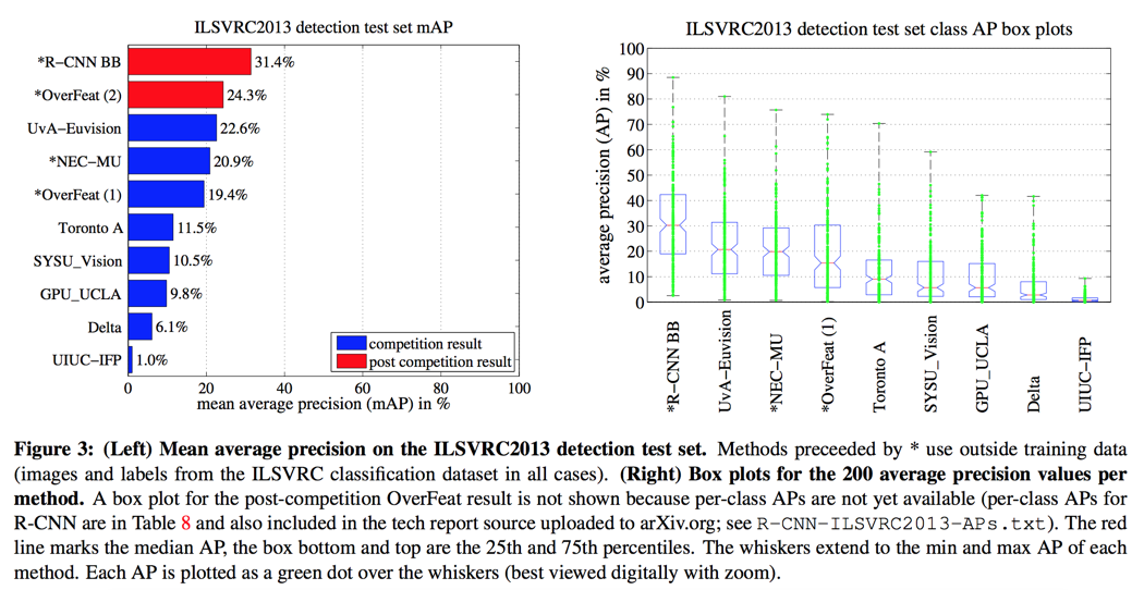
Visualization, Ablation and Modes of Error

visualizing learned features

We propose a simple (and complementary) non-parametric method that directly shows what the network learned

• compute the unit’s activations on a large set of held-out region proposals
• sort the proposals from highest to lowest activation
• perform non- maximum suppression

ablation studies

Performance layer-by-layer

without fine-tuning

features from fc7 generalize worse than features from fc6

with fine-tuning

The boost from fine-tuning is much larger for fc6 and fc7 than for pool5

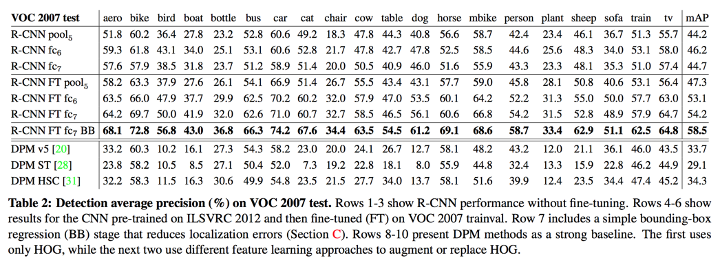
comparison to recent feature learning method

All R-CNN variants strongly outperform the three DPM baselines

network architectures

the choice of architecture has a large effect on R-CNN detection performance

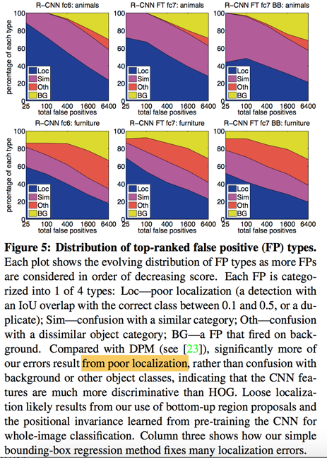
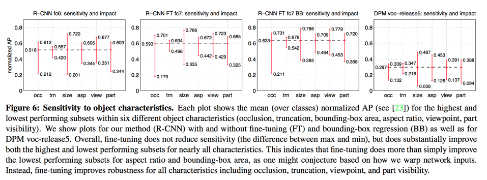
detection error analysis

we applied the excellent detection analysis tool from Hoiem et al.²³

bounding-box regression

we train a linear regression model to predict a new detection window given the pool5 features for a selective search region proposal

The input to our training algorithm is a set of N training pairs ${(P^i, G^i)}_{i = 1,\dots ,N}$ where $P^i = (P^i_x, P^i_y, P^i_w, P^i_h)$ specifies the pixel coordinates of the center of proposal $p^i$’s bounding box together with $P^i$’s width and height in pixels

ground-truth bounding box G is specified in the same way

our goal is to learn a transformation that maps a proposed box P to a ground-truth box G

we parameterize the transformation in terms of four functions $d_x(P), d_y(P), d_w(P), d_h(P)$

we can transform an input proposal P into a predicted ground-truth box $\hat G$ by applying the transformation:

• $\hat G_x = P_wd_x(P) + P_x$
• $\hat G_y = P_hd_y(P) + P_y$
• $\hat G_w = P_wexp(d_w(P))$
• $\hat G_h = P_hexp(d_h(P))$

we learn $w_*$ by optimizing the regularized least square objective:

$$w_* = \underset {\hat w_*} {argmin} \sum^N_i(t^i_* - \hat w^T_*\phi_5(P^i))^2 + \lambda ||\hat w_*||^2$$

where $\phi_5$ is pool5 features of proposal P and $t$ is calculated by ground-truth value

subtle issues:

• regularization is important($\lambda = 1000$)
• care must be taken when selecting which training pairs (P, G) to use(only use IoU >= 0.6)

we found that iterating does not improve results

qualitative results

skip

The ILSVRC2013 Detection Dataset

less homogeneous than PASCAL VOC

dataset overview

train (395,918), val (20,121), and test (40,152)

our general strategy is to rely heavily on the val set and use some of the train images as an auxiliary source of positive examples

region proposals

we followed the same region proposal approach that was used for detection on PASCAL

training data

we formed a set of images and boxes that includes all selective search and ground-truth boxes from val1 together with up to N ground-truth boxes per class from train

An initial experiment indicated that mining negatives from all of val1, versus a 5000 image subset (roughly half of it), resulted in only a 0.5 percentage point drop in mAP, while cutting SVM training time in half

The bounding-box regressors were trained on val1

validation and evaluation

we validated data on the val2 set

ablation study

essentially no difference between N = 500 and N = 1000

relationship to OverFeat

OverFeat can be seen (roughly) as a special case of R-CNN

• selective search vs multi-scale pyramid
• per-class bounding-box regressors vs single bounding-box regressor

It is worth noting that OverFeat has a significant speed advantage over R-CNN(9x faster)

Semantic Segmentation

CNN features for segmentation

we evaluate three strategies for computing features on CPMC regions:

• (full) ignores the region’s shape and computes CNN features directly on the warped window
• (fg) computes CNN features only on a region’s foreground mask
• (full+fg) simply concatenates the full and fg features

results on VOC 2011

• layer fc6 always outperforms fc7
• the context provided by the full features is highly informative even given the fg features

Conclusion

two insights:

• The first is to apply high-capacity convolutional neural networks to bottom-up region proposals in order to localize and segment objects
• The second is a paradigm for training large CNNs when labeled training data is scarce.

Reference

²³. D. Hoiem, Y. Chodpathumwan, and Q. Dai. Diagnosing error in object detectors. In ECCV. 2012. ↩