Wasserstein GAN

总结

• 文章首先说明了学习一个概率密度的传统方法使用KL散度
• 但是KL散度在两个低维流形的概率分布中不好使，因为他们没有无法忽视的重叠，从而散度是一个常数。通过加噪声可以补救这个问题，但是并不是一个好方法（对于GAN来说会使生成的图片模糊不清）
• 对于传统方法，目前的新方法是从一个固定分布$p(z)$随出一个随机变量$z$然后将$z$放入一个函数映射$g_\theta : z \rightarrow x$得到一个服从$P_\theta$分布的样本。
  • 这样做有两个好处，一个是这种方式可以更合更低维度的分布
  • 另外这种方式可以更加方便的生成新样本
• 接下来作者开始分析WGAN中使用Wasserstein距离代替原来JS散度的原因，从这种距离的性质入手
  • 如果$g_\theta$是连续的那么$W(P_r, P_\theta)$也是连续的
  • 如果$g$是K利普希茨连续，那么$W(P_r, P_\theta)$几乎在全部可导
  • 上述两条性质对于JS散度不成立，所以我们选用Wasserstein距离代替KL散度
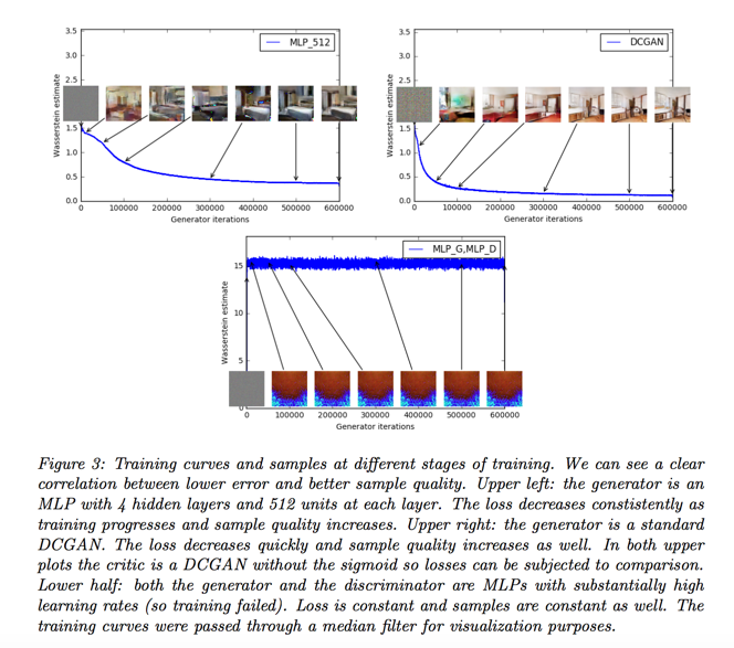
• 为了让$g_\theta$保持利普希茨连续，我们将网络中所有参数控制在[-0.01, 0.01]区间内
  • 这个数值不宜太大，否则会使收敛速度过慢
  • 不宜太小，否则可能会导致梯度消失
• 使用W距离后判别器损失函数为$-(f_w(x) - f_w(g_\theta(z)))$, 生成器损失函数为$-f_w(g_\theta(z))$
• 因为W距离连续可导，所以在交替训练的过程中可以将分类器训练至收敛，不必向以往一样两步分类器一步生成器
• WGAN的显著优势：
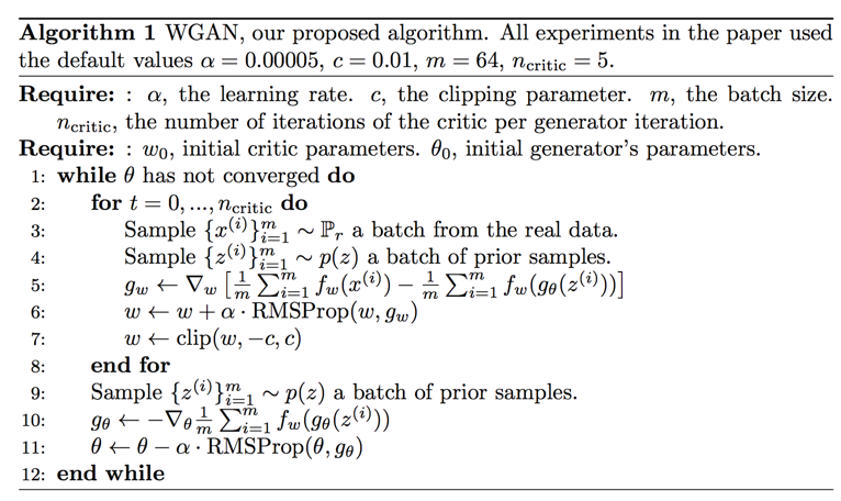
  • 不会模型坍塌——W距离连续得到的另外一个好处是不会导致模型坍塌；对于原始损失函数来说，判别器的输出是个二分类结果，那么对于最优的分类器来说，生成器的最终结果只能是坍塌即生成真实图像训练样本；换成W距离后，判别器输出的是距离，是回归问题，不会导致坍塌
  • WGAN提升了稳定性——由于我们在交替训练过程中可以把判别器训练到局部最优，判别器越精确，梯度也就越精确，训练也就越稳定
  • 有实际意义的损失函数——WGAN的生成器损失函数可以当做模型训练进度的可量化指标，不用向以往一样人肉观察生成出来的样本来做判别模型好坏的标准；但是需要注意不能拿这个指标衡量不同结构的模型
• optimizer的选择：训练的时候由于交替训练，损失函数不要使用基于动量的（如Adam）optimizer，改用RMSProp，一般在这种梯度不稳定的情况下表现的不错

Introduction

• when we learn a probability distribution, This is often done by defining a parametric family of densities $P_\theta (\theta \in R^d)$ and finding the one that maximized the likelihood on our data, this amounts to minimizing the Kullback-Leibler divergence $KL(P_r||P_g)$
• but It is then unlikely that the model manifold and the true distribution’s support have a non-negligible intersection
• the typical remedy is to add a noise term to the model distribution
• the added noise term is clearly incorrect for the problem, but is needed to make the maximum likelihood approach work

now:

• Rather than estimating the density of $P_r$, we varying $\theta : g_\theta(z) \rightarrow x$
• two advantages: this approach can represent distributions confined to a low dimensional manifold
• second, the ability to easily generate samples is often more useful than knowing the numerical value of the density

In this paper, we direct our attention on the various ways to measure how close the model distribution and the real distribution are

the contribution of this paper are:

• section 2, we provide a comprehensive theoretical analysis of how the Earth Mover (EM) distance behaves in comparison to popular probability distances and divergences used in the context of learning distributions
• section 3, we define a form of GAN called Wasserstein-GAN that mini- mizes a reasonable and efficient approximation of the EM distance, and we theoretically show that the corresponding optimization problem is sound
• section 4, we empirically show that WGANs cure the main training prob- lems of GANs.

Different Distance

• the total variation(TV) distance

$$\delta(P_r, P_g) = \underset {A \in \Sigma} {sup} |P_r(A) - P_g(A)|$$

• the Kullback-Leibler(KL) divergence

$$KL(P_r||P_g) = \int log(\frac {P_r(x)} {P_g(x)})P_r(x)d\mu(x)$$

• the Jensen-Shannon(JS) divergence

$$JS(P_r, P_g) = KL(P_r||P_m) + KL(P_g||P_m)$$

where $P_m$ is the mixture $(P_r + P_g) / 2$

• the Earth-Mover(EM) distance or Wasserstein-1

$$W(P_r, P_g) = \underset {\gamma \in \Pi(P_r, P_g)} {inf} E_{(x, y)\sim \gamma}[|| x - y ||] \label {1}$$

where $\Pi(P_r, P_g)$ denotes the set of all joint distributions $\gamma(x, y)$ whose marginals are respectively $P_r$ and $P_g$

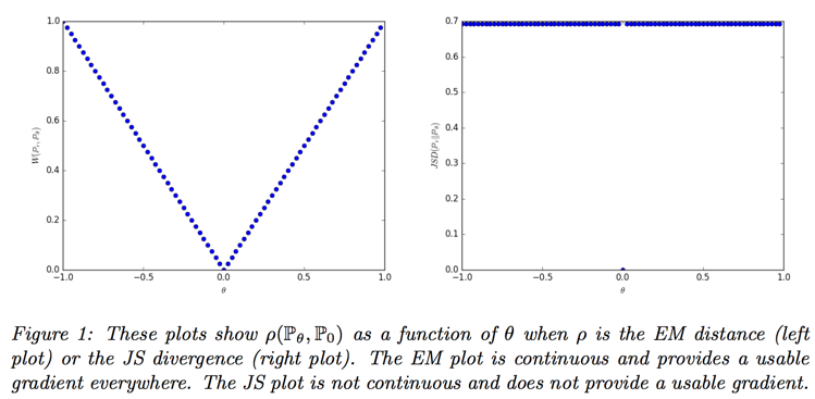
use EM distance as lose function:

• if g is continuous in $\theta$, so is $W(P_r, P_\theta)$
• if g is locally Lipschitz and satisfies regularity assumption, then $W(P_r, P_\theta)$ is continuous everywhere, and differentiable almost every where
• statement 1 and 2 are false for the JS divergence and KLs

All this shows that EM is a much more sensible cost function for our problem

Wasserstein GAN

the infimum of Wasserstein distance is highly intractable, but Kantorovich-Rubinstein duality tells us that

$$W(P_r, P_\theta) = \underset {||f||_L \le 1} {sup} E_{x \sim P_r}[f(x)] - E_{x \sim P_\theta}[f(x)]$$

we have

$$\nabla_\theta W(P_r, P_\theta) = - E_{z \sim p(z)}[\nabla_\theta f(g_\theta(z))] \tag 1$$

to roughly approximate a appropriate function, something that we can do is train a neural network parameterized with weights w lying in a compact space W and then backprop through equation(2)

in order to have parameters w lie in a compact space, something simple we can do is clamp the weights to a fixed box (say $W = [−0.01, 0.01]^l$) after each gradient update

means that we can (and should) train the critic till optimality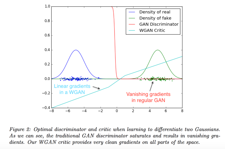

the fact that we can train the critic till optimality makes it impossible to collapse modes

Empirical Results

two main benefits of WGANs:

• a meaningful loss metric that correlates with the generator’s convergence and sample quality
• improved stability of the optimization process

Experimental Procedure

dataset: LSUN-Bedrooms dataset
baseline: DCGAN

Meaningful loss metric

our first experiment illustrates how this estimate correlates well with the quality of the generated samples

the constant scaling factor that depends on the critic’s architecture means it’s hard to compare models with different critics

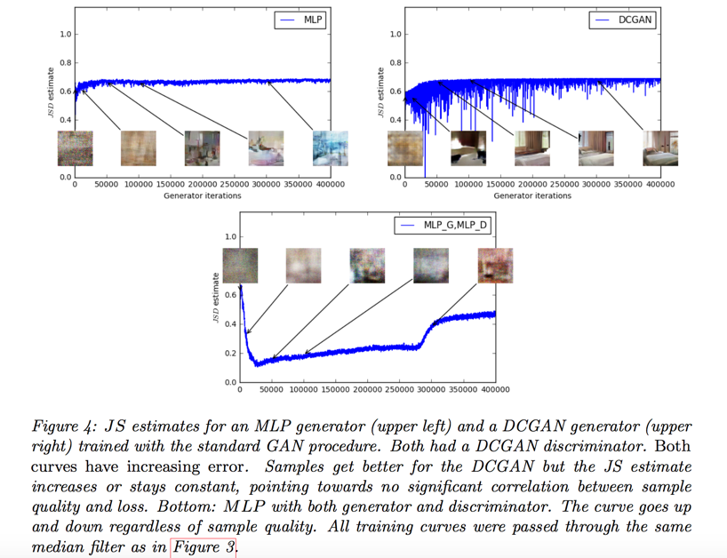
JS divergence has no significant correlation between sample quality and loss

don’t use momentum based optimizer, otherwise training process will be unstable, use RMSProp instead

improved stability

• one of the benefits of WGAN is that it allows us to train the critic till optimality the better the critic, the higher quality the gradients we use to train the generator
• another benefit is that WGANs are much more robust than GANs when one varies the architectural choices for the generator
  

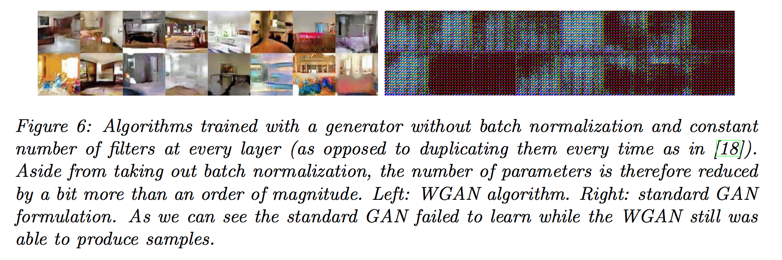
• in no experiment did we see evidence of mode collapse for the WGAN algorithm

Related Work

skip…

Conclusion

• improve the stability of learning
• no mode collapse
• provide meaningful learning curves useful for debugging and hyperparameter searches