总结
- 生成对抗网络由生成器G和分类器D组成,生成器G接受噪音生成样本,D负责区分这些样本是否是由D生成出来的
- D和G共同优化目标函数$\underset {G} {min} \underset {D} {max} V(D,G) = E_{x \sim p_{data}(x)}[log(D(x))] + E_{x \sim P_{g_z(z)}}[log(1 - D(g(z)))]$ 一个是让值尽量大,一个是让值尽量小,即所谓“对抗”
- 该目标函数会在$p_g = p_{data}$处收敛到最优,即生成分布与训练数据分布完全一致函数值为$-log4$
- 关于收敛性的证明:一个凸函数集合的上界的次梯度(可导的时候等于梯度)完全包含最后函数的梯度,所以在求导做梯度下降的时候整体仍然按照凸函数的性质收敛
- 使用Gaussian Parzen window(youtube视频)方法对模型进行评估, Parzen Window 其实是用已有数据到待测数据点的“距离”平均值来表示待测点出现在已有数据表示的分布上的概率(或者说在已有数据拟合出的概率密度函数上的值)
- 通用概率密度函数$P(x) = \frac {1} {n}\sum_{i = 1}^{n}\frac {1} {h^d}K(\frac {x - x_i} {h})$
- Parzen window中的核函数可以有多种,使用Gaussian核的就叫做Gaussian Parzen window$P(x) = \frac {1} {n} \sum^n_{i = 1}\frac {1} {h\sqrt {2\pi}^d}exp(-\frac 1 2(\frac {x - x_i} {h})^2 )$
- 算出概率之后再过一遍$score = -log(1 - P(x))$(猜测)
- 优点
- 不使用马尔科夫链
- 训练模型的时候不需要inference
- 可拟合sharp的分布
- 训练样本并不直接作用于G的训练,保证参数独立
- 可使用多种模型拟合G和D
- 缺点
- G和D需要同步训练(两次D一次G)
- 没有$p_g(z)$分布的显示表示
Abstract
propose a new framework for estimating generative models via adversarial process
simultaneously train two models:
- a generative model G
- a discriminative model D
a unique solution exists, with G recovering the train data distribution and D equal to $\frac 1 2$ everywhere
Introduction
a discriminative model that learns to determine whether a sample is from the model distribution or the data distribution. The generative model can be thought of as analogous to a team of counterfeiters
Relate Work
- restricted Boltzmann machines(RBM)
- deep Boltzmann machines(DBMs)
- deep belief networks(DBNs)
- score matching
- noise-contrastive estimation
- generative stochastic network
Adversarial nets
G is a differentiable function to output a generate data by $G(z;\theta_g)$
D is a multilayer perce ptron $D(x;\theta_d)$ to output a single scalar that represent whether a data is fabricated by G
D and G play the following two-player minimax game with value function $V(G, D)$
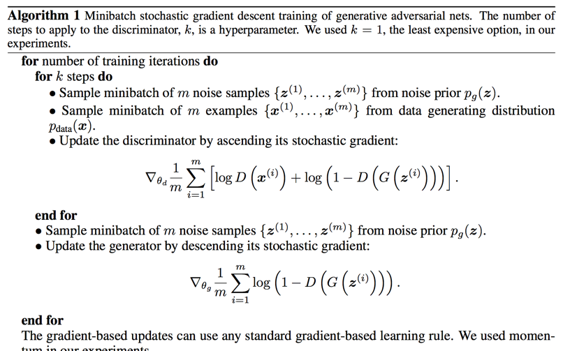
we alternate between k steps of optimizing D and one step of optimizing G
Early in learning, when G is poor $log(1 - D(G(z)))$ saturates. we use $\underset {G} {max} logD(G(z))$ instead. It’s provides much stronger gradients early in learning
Theoretical Results
Global Optimality of $p_g = p_{data}$
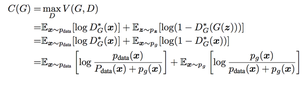
the global minimum of the virtual training criterion $C(G)$ is achieved if and only if $p_g = p_{data}$. At that point, $C(G)$ achieves the value - $log4$
Since the Jensen–Shannon divergence between two distributions is always non-negative and zero only when they are equal
Convergence of Algorithm 1
If G and D have enough capacity, and at each step of Algorithm 1, the discriminator
is allowed to reach its optimum given G, and $p_g$ is updated so as to improve the criterion
proof:
The subderivatives of a supremum of convex functions include the derivative of the function at the point where the maximum is attained
一个凸函数集合的上界的次导数包含达到最大值的函数的导数
看不懂……
Experiments
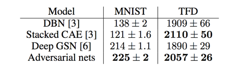
database:
- MNIST
- TFD
- CIFAR-10
activation:
generator use mixture of rectifier linear and sidmod as activations; discriminator use maxout activation
We estimate probability of the test set data under $p_g$ by fitting a Gaussian Parzen window to the samples generated with G and reporting the log-likelihood under this distribution
Advantages and disadvantages
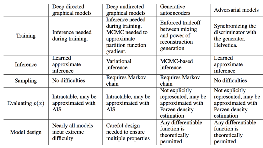
disadvantages:
- there is no explicit representation of $p_g(x)$
- and that D must be synchronized well with G during training (in particular, G must not be trained too much without updating D, in order to avoid “the Helvetica scenario” in which G collapses too many values of z to the same value of x to have enough diversity to model $p_{data}$)
advantages:
- Markov chains are never needed
- no inference is needed during learning
- a wide variety of functions can be incorporated into the model
- generator network not being updated directly with data examples, but only with gradients flowing through the discriminator
- they can represent very sharp, even degenerate distributions
Conclusions and future work
extensions in future:
- A conditional generative model $p(x | c)$ can be obtained by adding c as input to both G and D
- Learned approximate inference can be performed by training an auxiliary network to predict z given x
- Semi-supervised learning