总结
- 本文的主旨是将生成proposal的过程也使用神经网络处理,并且共享了classification的中间卷积结果,大大减少了proposal过程的用时
RPN网络结构
- 用一个n*n(本文用3)的卷积核在classification的最后一层卷积出来的feature map上滑动
- 以每个feature为中心生成3(不同尺寸)*3(不同比例)的定长proposal 特征vector(在训练时与图片边界产生交叉的proposal丢弃)
- 然后在这个vector后面接两个1*1卷积,得出两组结果
- 一组表示这个proposal有待检测物体的概率(2个数 softmax)
- 一组表示边界框的位置(4个数)
- 根据有物体的概率做NMS(阈值0.7)
- 这种生成proposal的方式具有平移不变性
网络训练
- 损失函数和Fast-RCNN一样,也是分类损失和回归损失的结合
- 构造batch的时候尽量正负样本比1:1
共享参数
- 由于做detection的时候要求proposal方式的固定的,这就导致了(暂时)没法让这两个流程一起训练
- 作者给出了一个4步训练流程
- 先单独训练RPN
- 然后用RPN给出的proposal单独训练Fast-RCNN
- 然后用Fast-RCNN的中间卷积结果,单做RPN的滑动feature map,冻结中间卷积结果,fine-tuning RPN
- 然后冻结中间卷积结果,fine-tuning Fast-RCNN的卷积结果后面几层(fc层)
简化实验
简化一些功能,通过最终效果推导该功能的效果
| 简化功能 | mAP变化 | 原因 |
|---|---|---|
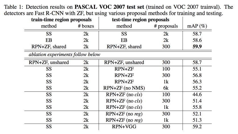
| 不共享参数 | 59.9->58.7 | 共享训练的第三步,提高了RPN的效果 |
| 在训练过程中用SS代替RPN,去除RPN对detection部分的影响(下面的实验都是) | 59.5->56.8 | 由于训练和测试时proposal的不一致 |
| 只用top100的proposal | 56.8->55.1 | 只下降了一点,证明RPN的精确度很高 |
| 不用NMS | 56.8->55.2 | 证明NMS不仅加快了速度而且不会降低mAP |
| 去除RPN的cls输出, 随机取top1k | 56.8->55.8 | 基本没动,与下面实验对比 |
| 去除RPN的cls输出,随机取top100 | 56.8->44.6 | cls输出与proposal是否包含物体高度相关 |
| 去除RPN的reg输出 | 56.8->52.1 | 物体框的精度主要靠reg输出修正来提高 |
| 使用更强大的网络 | 56.8->59.2 | 网络结构对结果的影响很大 |
VOC测试结果
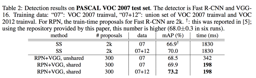
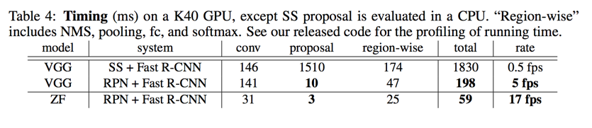
- time: 198ms
- VOC 2007
- 07 data: 69.9%
- 07+12 data: 73.2%
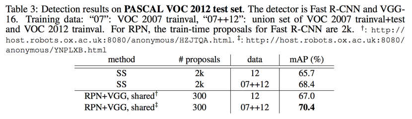
- VOC 2012
- 12 data: 67.0%
- 07+12 data: 70.4%
Abstract
we introduce a Region Proposal Network (RPN) that shares full-image convolutional features with the detection network, thus enabling nearly cost-free region proposals
Introduction
proposals are the computational bottleneck in state-of-the-art detection systems
re-implement region proposal for the GPU. This may be an effective engineering solution
we show that an algorithmic change—computing proposals with a deep net
our observation is that the convolutional (conv) feature maps used by region-based detectors
- one that encodes each conv map position into a short (e.g., 256-d) feature vector
- at each conv map position, outputs an objectness score and regressed bounds for k region proposals
Related Work
skip
Region Proposal Networks
a Region Proposal Network (RPN) takes an image (of any size) as input and outputs a set of rectangular object proposals, each with an objectness score
- slide a small network(n * n) over the conv feature map output by the last shared conv layer
- this vector is fed into two sibling fully-connected layers
- a box-regression layer (reg)
- a box-classification layer (cls)
- this architecture is naturally implemented with an n × n conv layer followed by two sibling 1 × 1 conv layers (for reg and cls, respectively)
- n = 3 in this paper
")
translation-invariant anchors
while predict k region proposals, there are
- 4k outputs in reg layer
2k(softmax)/k(regression) outputs in cls layer
we use 3 scales and 3 aspect ratios, yielding k = 9 anchors
this approach is translation invariant
a loss function for learning region proposals
positive label:
- the anchor/anchors with the highest Intersection-over-Union (IoU) overlap with a ground-truth box
- an anchor that has an IoU overlap higher than 0.7 with any ground-truth box
negative label:
- IoU ratio is lower than 0.3 for all ground-truth boxes
drop other anchors
loss function for an image is defined as:
each regressor is responsible for one scale and one aspect ratio
optimization
we randomly sample 256 anchors in an image where the sampled positive and negative anchors have a ratio of up to 1:1
sharing convolutional features for region proposal and object detection
describe an algorithm that learns conv layers that are shared between the RPN and Fast R-CNN
Why can’t we push them together
- Fast R-CNN training depends on fixed object proposals
- training simultaneously maybe not converge
4-step training algorithm:
- we train the RPN as described above
- we train a separate detection network by Fast R-CNN using the proposals generated by the step-1 RPN
- we use the detector network to initialize RPN training, but we fix the shared conv layers and only fine-tune the layers unique to RPN
- Finally, keeping the shared conv layers fixed, we fine-tune the fc layers of the Fast R-CNN
implementation details
multi-scale feature extraction may improve accuracy but does not exhibit a good speed-accuracy trade-off
box side size:
- 128
- 256
- 512
aspect ratio
- 1:1
- 1:2
- 2:1
Question:
- how to handle the anchor boxes that cross image boundaries?
Answer:
- during training, we ignore all cross-boundary anchors so they do not contribute to the loss
- during testing, however, we still apply the fully-convolutional RPN to the entire image
adopt non-maximum suppression and fix the IoU threshold for NMS at 0.7
Experiments
ablation experiments
shared to unshared:
reduces the result slightly to 58.7%
in the third step when the detector-tuned features are used to fine-tune the RPN, the proposal quality is improved
SS in training & RPN in testing:
leads to an mAP of 56.8%
because of the inconsistency between the training/testing proposals
use top 100 proposals only:
leads to a competitive result (55.1%)
RPN proposals are accurate
without NMS:
mAP: 55.2%
NMS does not harm the detection mAP and may reduce false alarms
without cls:
randomly sample N proposals
top 100’s mAP: 44.6%
shows scores account for the accuracy
without reg:
mAP drops to 52.1%
this suggests that the high-quality proposals are mainly due to regressed positions
more powerful networks:
The mAP improves from 56.8% (using RPN+ZF) to 59.2% (using RPN+VGG)
detection accuracy and running time of VGG-16
VOC 07:
VOC 12:
run time:
analysis of recall-to-IoU
It is more appropriate to use this metric to diagnose the proposal method than to evaluate it
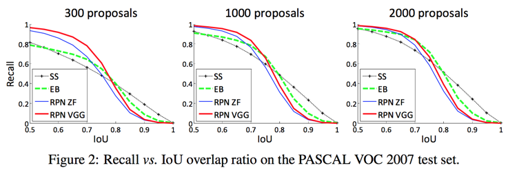
the RPN method behaves gracefully when the number of proposals drops from 2k to 300
one-stage detection vs. two-stage proposal + detection
- class-specific detection pipeline
- class-agnostic proposals and class-specific detections
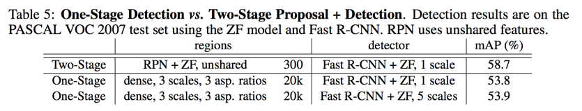
the one-stage system has an mAP of 53.9%. this is lower than the two-stage system (58.7%) by 4.8%
the one-stage system is slower as it has considerably more proposals to process
Conclusion
skip