Factorization Machines

• Factorization Machine are a new model class that combines the advantages of Support Vector Machines
• able to estimate interactions even in problems with huge sparsity
• dual form is not necessary, estimate model parameters directly

INTRODUCTION

the advantages of FM:

• FMs allow parameter estimation under very sparse data where SVMs fail
• FMs have linear complexity, can be optimized in the primal and do not rely on support vectors like SVMs
• FMs are a general predictor that can work with any real valued feature vector. In contrast to this, other state-of-art factorization models work only on very restricted input data

PREDICTION UNDER SPARSITY

assume we have the transaction data of a movie review system. here feature vectors can be created as follow: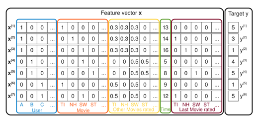

FACTORIZATION MACHINES

factorization Machine Model

model equation

$$\hat y(x) := w_0 + \sum_{i = 1}^n w_ix_i + \sum_{i = 1}^n\sum_{j = i + 1}^{n}<v_i, v_j>x_ix_j$$

where in $<\cdot , \cdot>$ is dot product of two vectors

• $w_0$ is the global bias
• $w_i$ models the strength of the i-th variable
• $\hat w_{i,j} := $ models the interaction between the i-th and j-th variable. Instead of using an own model parameter $w_{i,j}$ for each interaction, the FM models the interaction by factorizing it. this is the key point which allow high quality parameter estimates of higher-order interaction(d >= 2) under sparsity

Expressiveness

FMs can express any interaction matrix W if k is chosen large enough. Nevertheless in sparse settings, typically a small k should be chosen because there is not enough data to estimate complex interaction matrix W

Parameter Estimation Under Sparsity

FMs can estimate interactions even in sparsity data well because they break the independence of the interaction parameters by factorizing them

computation

straight forward computation of equation 1 is in $O(kn^2)$
with reformulating it drops to linear runtime

after follow reformulation complexity of computation si down to$O(kn)$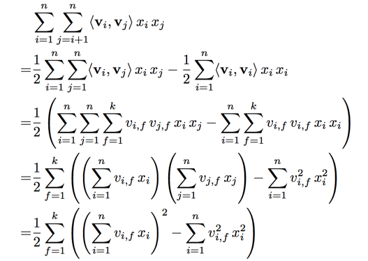

moreover we have only to compute non-zero elements, thus the complexity is down to $O(k\overline m_D)$ $\overline m_D = 2$ for typical recommender systems

Factorization Machines as Predictors

FM can be applied to a variety of prediction tasks

• Regression
• Binary classification
• Ranking

regularization terms like L2 are usually added to optimization objective to prevent overfitting

Learning Factorization Machines

the gradient of the FM model is: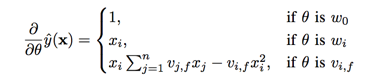

$\sum_{j=1}^nv_{j,f}x_j$ is independent of i and thus can be precomputed

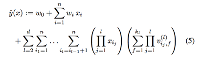
d-way Factorization Machine

the two-way FM describe so far can easily be generalized to a d-way FM:

Summary

two main advantages:

• The interactions between values can be estimated even under high sparisity. Especially, it is possible to generalize to unobserved interactions
• The number of parameters as well as the time for prediction and learning is linear.

FMs vs SVMs

SVM model

In the following, we discuss the relationships of FMs and SVMs by analyzing the primal form of the SVMs

linear kernel

kernel: $K(x, z) = 1 + $
mapping: $\phi(x) = (1, x_1, \dots, x_n)$
SVMs:

$$\hat y(x) = w_0 + \sum_{i = 1}^{n}w_ix_i$$

is identical to a FM of degree d = 1

polynomial kernel

kernel: $K(x,z) = ( + 1)^2$
mapping: $\phi(x) = (1, \sqrt2x_1, \dots, \sqrt2x_n,$

$$x_1^2, \dots, x_n^2,$$ $$\sqrt2x_1x_2, \dots, \sqrt2x_1x_n, \sqrt2x_2x_3, \dots, \sqrt2x_{n-1}x_n)$$

SVMs:

$$\hat y(x) = w_0 + \sqrt2\sum_{i = 1}^nw_ix_i + \sum_{i = 1}^{n}w_{i,i}^{(2)}x_i^2 + \sqrt2\sum_{i = 1}^n\sum_{j = i +1}^nw_{i,j}^{(2)}x_ix_j$$

is similar to a FM of degree d = 2

• all interaction parameters w_{i, j} of SVMs are completely independent
• the interaction parameters of FMs are factorized

parameter Estimation Under Sparsity

in the case of collaborative filtering with user and item indicator variables. The feature vectors are sparse and only two elements are non-zero

linear SVM

model is equivalent to

$$\hat y(x) = w_0 + w_u +w_i$$

As this model is very simple, the parameters can be estimated well even under sparsity, nevertheless the empirical prediction quality is low

Polynomial SVM

model is equivalent to

$$\hat y(x) = w_0 + \sqrt2(w_u + w_i) + w_{u,u}^{(2)} + w_{i,i}^{(2)} + \sqrt2w_{u,i}^{(2)}$$

the interaction item $w_{u,i}^{(2)}$ has at most one observation in the training data. And thus the polynomial SVM can make no use of any 2-way interaction for predicting.so the Polynomial SVM cannot provide better estimations than linear SVM

summary

• FMs can be estimated well even under sparsity. SVMs can not
• FMs can be directly learned in the primal. Non-linear SVMs are usually learned in the dual
• The model equation of FMs is independent of the training data. Prediction with SVMs depends on parts of the training data

FMs vs. Other Factorization Models

Matrix and Tensor Factorization

MF is the simple version model of FM, which only has interaction parts

SVD++

SVD++ model:

$$w_0 + w_u + w_i + q_i^T(p_u + |N(u)|^{-\frac {1} {2}}\sum_{j \in N(u)}y_j)$$

A FMs can mimic this model by using the following input data: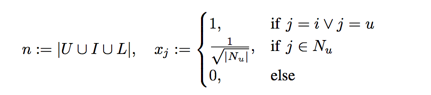

now the input data set is like this:

$$(u, i, N_{u_1}, N_{u_2}, \dots, N_{u_l})$$

the prediction result resolved to three parts:

• bias parts: $w_0$
• linear parts: $w_u + w_i + w_l$
• interaction parts: $, , , <\sum_j^lN_{u_j}, \sum_{k = j+1}^lN_{u_k}>$

re-rank element according to SVD++: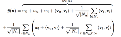

PITF for Tag Recommendation

The problem of tag prediction is defined as ranking tags

input data set is:

the prediction result reolved to three parts

• bias parts: $w_0$
• linear parts: $w_u + w_i + w_t$
• interaction parts: $ + + $

in the tag recommendation situation, only one difference between two competitor, $vt$

the FM model is equivalent to:

$\hat y(x) = w_t + + $

PITF and FM are almost identical except

• FM model has a bias term
• the factorization parameters for the tags $v_t$ are shared for the FM model but individual for the original PITF model

the figure shows empirically that both models also achieve comparable prediction quality for this task

Factorized Personalized Markov Chains

input date set is: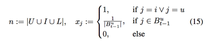

where $B_t^u \subseteq L$ is the set of all items a user u has purchased at time t

the prediction: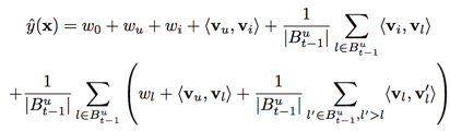

only score differences between $(u, i_A, t)$ and $(u, i_B, t)$ are used in the prediction is item term

FM model is equivalent to:

$$\hat y(x) = w_i + <v_u, v_i> + \frac 1 {B_{t-1}^u}\sum_{l \in B_{t-1}^u}<v_i, v_l>$$

difference between FPMC and FMs

• bias
• share item vector

summary

• through m parts joining into a whole matrix, FM is identical to MF
• FM can mimic other specialized models(such as SVD++, PITF, FPMC) well